Phase Field Techniques
Phase field techniques are a powerful numerical tool for the simulation of many problems in mechanics and materials science. An order parameter is the primary unknown field which describes, e.g., a phase distribution (in case of phase transitions or phase separation) or a domain distribution (in case of ferroeletrics, ferromagnetics). The evolution of the order parameter is goverened by a kinetic relation, which if often assumed to be of either Cahn-Hilliard type (when the average of the order paramter across the simulatino domain is conserved, e.g., in case of phase separation where the mean concentration remains constant) or of Allen-Cahn-type (when the average may also evolve in a diffusive fashion, e.g., in case of ferroelectric switching where one domain may grow while another disappears). The simulation of processes via phase field techniques enables us to study both equilibrium microstructures found in materials as well as, to some extent, the kinetics of microstructural evolution processes; the latter still being a somewhat open challenge. We develop new theoretical models and associated numerical techniques to simulate such processes.
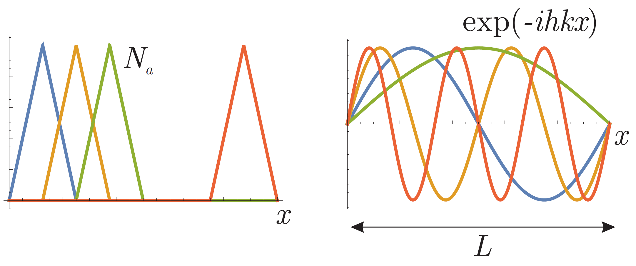
When simulating a representative unit cell at a material's microscale, we often assume periodic boundary conditions, for which a spectral solution approach is an efficient alternative to using classical techniques such as finite elements. The key idea is to replace the piecewise-polynomial interpolation functions of finite elements by periodic (cose/sine-type) interpolation functions that have the periodicity of the solution built in (see the schematic below). An added benefit is that such periodic homogenization approaches, which date back to early work by P. Suqet and collaborators, have as their only expensive numerical steps a discrete Fourier transform and its inverse. Depending on the particular scheme, tThere is no need to compute or store consistent tangent matrices, while still solving the implicit quasistatic boundary value problem, which facilitates the simulation at very high resolution in 3D (where finite elements usually run into storage and efficiency issues).
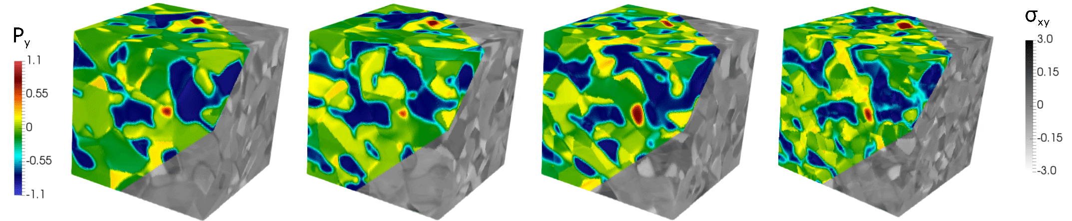
Spectral solution strategies in combination with heterogeneous material properties, for instance jumps in the dielectric and elastic constants, or differently oriented grains in a polycrystal, result in ringing artefacts better known as Gibbs phenomenon, see Fig. (a) below, where this effect is demonstrated for linear elasticity on a 1D rod with a soft core and stiff end sections. Such high-frequency oscillations near discontinuities are caused by non-uniform convergence of the truncated Fourier series. In order to overcome the Gibbs phenomenon, we use finite difference stencils to approximate gradients [1], which are asymptotically stable under h-refinement and hence, ensure that the derivative in a domain remains bounded. The disadvantage of this approach is that the pointwise convergence of the spectral method reduces from exponential to the order of the finite difference stencil. In general, higher-order or compact finite difference schemes are favoured, for example an 8th-order finite difference stencil is used to simulate the ferroelectric microstructure for an increasing number of grains (or discontinuities), see Fig. (b) below.
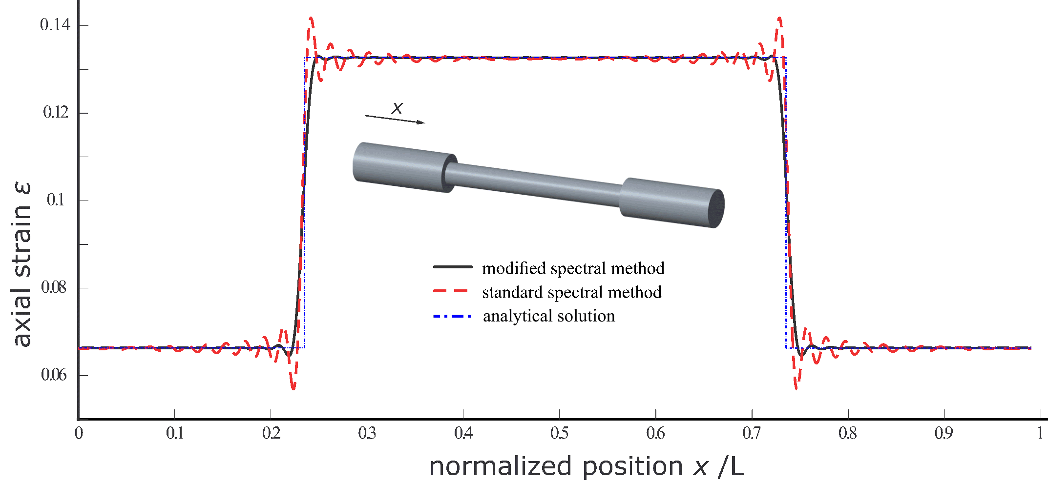
Spectral solution strategies in combination with heterogeneous material properties, for instance jumps in the elastic or other physical properties within the simulation doamin, or differently oriented grains in a polycrystal, result in ringing artefacts associated with the well-known Gibbs phenomenon, see below. In this figure, the ringing effect is demonstrated for a linear elastic 1D rod whose cross-section changes discontinuously (the bar is divided into three cross-sections, each having a distinct but constant cross-section). Without any correction, we observe high-frequency oscillations near the discontinuities, which are caused by the non-uniform convergence of the truncated Fourier series (after all, in any numerical scheme we cannot work with the exact, infinite Fourier series but can retain only a finite number of terms or grid points, see external page Vidyasagar et al., JMPS 2017.
In order to overcome the ringing artifacts, we use finite difference stencils to approximate spatial gradients before taking a Fourier transform. This approximation is asymptotically consistent under h-refinement and hence ensures that the spatial gradients in a domain remain bounded. The disadvantage of this approach is that the pointwise convergence of the spectral method reduces from exponential to the order of the finite difference stencil. As a major advantage, ringing artifacts are suppressed and the solution at discontinuous is smeared out over a numerical finite width which only depends on the spatial grid resolution and not on any physical length scales involved in the model (see external page Vidyasagar et al., CMAME 2018).
In general, higher-order or compact finite-difference stencils are favoured, for example an 8th-order finite difference stencil was used to simulate the ferroelectric microstructure for an increasing number of grains (or discontinuities) in a polycrystal, as shown above. Similar techniques are being applied to simulating plasticity and microstructural phenomena in magnesium alloys.
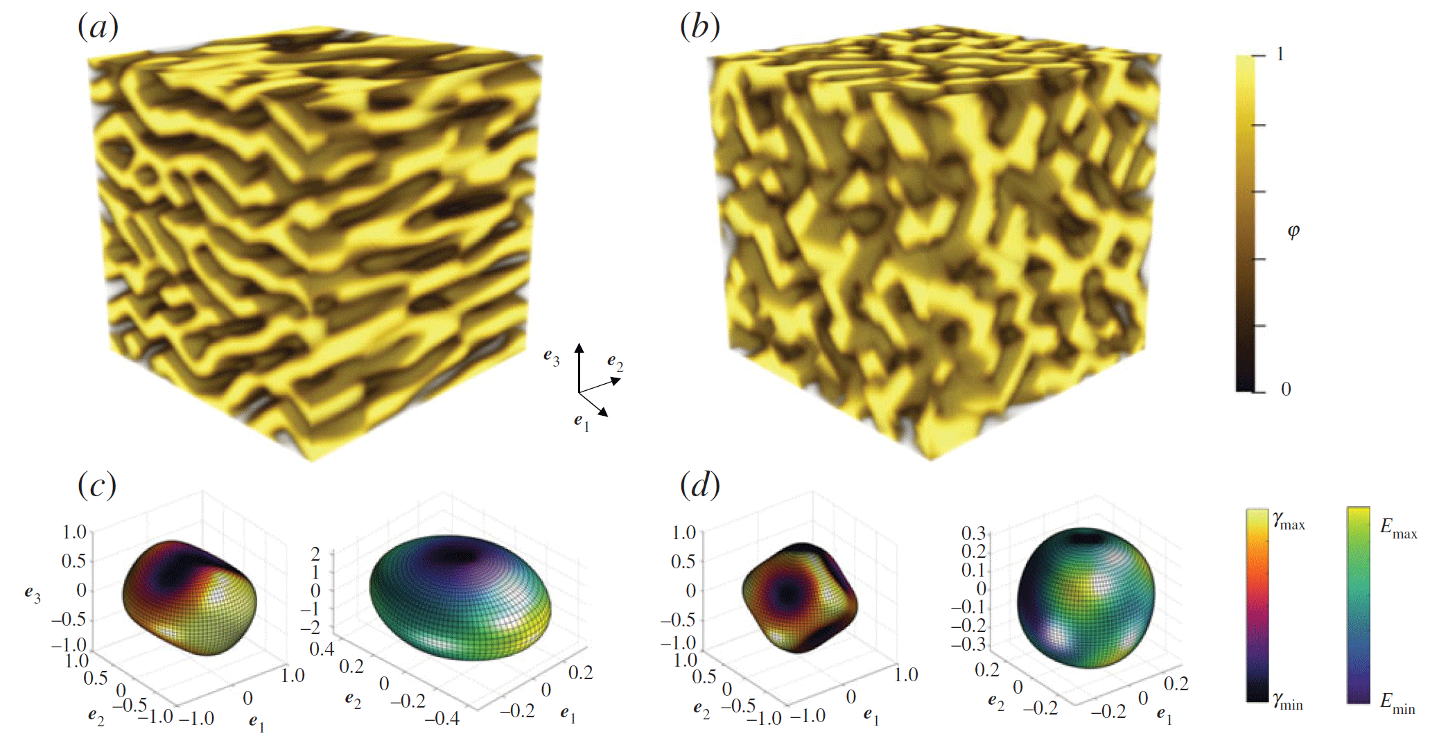
Besides modeling microstructures in metals and ceramics, we have also applied such techniques to, e.g., spinodal phase separation (see above). The scheme is beneficial not only for describing the time-dependent phase separation process within a reprentative unit cell but also for computing the effective properties of the resulting cellular architecture, such as the resulting elastic surfaces (shown below; these illustrate the direction dependent Young's modulus of the medium), see external page Vidyasagar et al., PRSA 2018 or read more about spinodal decomposition.